Currently in Europe, sun protection products must follow many recommendations and although they are not law, compliance is expected from the cosmetic industry by regulators, consumers and the industry itself. For example, the European Commission and Colipa recommend that products provide both UVB and UVA protection, with an SPF ratio of at least one-third. SPF claims are organized into four categories: low SPFs of 6 and 10; medium SPFs of 15, 20 and 25; high SPFs of 30 and 50; and very high SPFs of 50+.1, 2
In relation, in the United States in 2007, the US Food and Drug Administration (FDA) proposed an amendment to its Final Monograph relating to sun protection.3 The proposed rules are different than Europe’s for UVA but are similar in terms of SPF. The FDA has proposed: replacing its current category descriptors of minimal and moderate respectively with the terms low, meaning SPF 2 to < 15, and medium, meaning SPF 15 to < 30; and increasing the labeled SPF value to 50 for SPF 30–50, and 50+ for SPF 50+.
SPF is assessed based on the biological marker erythema, which is caused by a certain portion of UV radiation and is a generally accepted benchmark by which consumers choose sunscreen products. So while companies should test sunscreen products throughout the development process to ensure the desired SPF level is maintained, many also measure SPF in vivo during the development phase since the final SPF claimed is obtained in vivo. Oftentimes, in order to cut the costs of in vivo testing, companies reduce the number of volunteers from 10 to 5.
The purpose of this article is to provide product developers with a guide for interpreting in vivo SPF results. Values including the mean, standard deviation and confidence intervals are related to probability concepts that are often misunderstood or misinterpreted, which can lead to serious consequences since the screening value of the in vivo SPF has a direct effect on the product’s further development. Product developers should thus consider whether two SPF results being compared are similar.
All of these parameters will be explained and discussed here. From the SPF mean and standard deviation, the authors will show how to calculate the confidence percentage if a result obtained is different from the claimed SPF mean. Step by step calculation will be given in order to compare two means, and the impact of a decrease from 10 to 5 volunteers on the results will be discussed. Tools for decision support also will be communicated.
Reading and Interpreting In vivo Results
In vivo results given by test institutes mainly include statistical calculations such as the: mean, standard deviation, confidence interval (CI), lower limit of CI, upper limit of CI, standard error mean (SEM) and labeled SPF; and although product developers are likely familiar with this information, it is not uncommon for them to rely only on the claimed SPF. However, all of these factors are important and provide significant details that allow for a more accurate analysis of the results to make more appropriate product development decisions.
Approaches to interpreting the results, in this article, are based on two important assumptions—first, that the sampling taken by the testing lab is accurately representative of the population described in Colipa’s International Sun Protection Factor Test Method.4 This responsibility lies with the test institute but most facilities are fully compliant with the guidelines. The second assumption is that the statistics given in the report are issued from a normally distributed sampling.
This second point was investigated by the authors on 12 randomly selected samples from a one-year set of internal reports with claimed SPF levels from 6 to 50+. Using appropriate statistical tests, i.e., normal quantile plots, outlier analyses and Shapiro and Wilk’s W-testa, the authors observed normality across this sampling, with p values ranging from 0.07 to 0.78; and as is generally known, the p value must be greater than 0.05. Since normally distributed results were consistent in the data set, the authors assumed this to be the case in further in vivo tests.
Arithmetic average: To the product formulator, the arithmetic average of SPF values gives an indication of what the real SPF value could be, which can be used in deciding whether to continue a given product’s development or to reformulate. The arithmetic average of a data set hides the value of both the most frequently observed value and the real value; the data set is thus separated into two equal classes of the observed population—50% with a higher SPF, and 50% with a lower SPF than the mean of the population. If the SPF of the whole consumer population could be evaluated, this value would represent the real mean SPF.
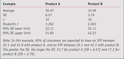
In the simulated evaluation shown in Table 1, calculations comparing two products on 10 volunteers estimate that the SPF mean for product A is 36.97 and B is 33.69. In this example, the normality assumption has been accepted because in the two cases, the Shapiro and Wilk’s Test concludes there will be a greater than 0.05 risk (0.55 for product A and 0.41 for product B); note that typically, a risk greater than 0.05 is considered too high.
Standard deviation: To the product formulator, the standard deviation of SPF values gives an indication of a pool of heterogeneity between consumer SPF results and uncertainty on measurements, and can be used to estimate the global uncertainty of in vivo results. Standard deviation (SD) represents the average distance of one consumer’s measured SPF results from the mean of all consumers in the test population. According to the normal law shape, Table 2 summarizes the areas of the bell curve in which SPF data collected from a population of consumers would be expected to be distributed.
The coefficients given in Table 2—i.e., 1, 2 and 3, are useful for a quick approximation of the distribution intervals of the population. However, since product developers typically work with small size samples (n < 30), it is more relevant to use the Student’s t-value5 associated with the sample size in place of coefficients 1, 2 and 3. For example, for 95% with 10 volunteers, the t-value equals 2.262 (see simulated example in Table 3).
In this example, 95% of consumers are expected to obtain an SPF between 22.1 and 51.8 with product A and an SPF between 25.1 and 42.3 with product B. Readers should note that these distribution intervals (DI) do not draw conclusions on the rankings of products, they only give the range of SPF observed on the whole population of consumers sampled. These intervals could change with an increase in the sample size or a new test due to the changing average and/or SD. Later, this article will show how to rigorously compare the results of two products obtained from different tests or even test methods.
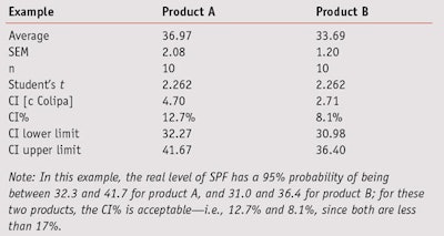
Confidence interval: To the product formulator, the CI of SPF values gives an indication of the area in which the real SPF is assumed to be, and can be used to estimate the real SPF lower limit (to be used in product claims). CI represents the 95% Half Range (HR) and is also called the uncertainty (u). If the same SPF investigation previously described is evaluated with another set of volunteers, there is a 95% chance that the result, as well as the real level of SPF, will be in the interval given by the average + u; note that in the Colipa guidelines, the letter c is used in place of u.
In in vivo SPF reports, the uncertainty value is expressed as a percentage of the mean CI%; and since 95% is the confidence level in this example, 17% is an acceptable level of the half interval, expressed as a percentage of the mean SPF, per Colipa guidelines. Another way to express this result is given by the two limits of the CI—lower and upper.
Comparing SPF Variability
It is important that product developers compare the variability of the results from testing two product samples to choose the most appropriate test to compare their means, as is explained further below. In order to compare the variability of SPF products tested in vivo, or those assessed via different methods—e.g., in vivo and in vitro, the SEM is provided and is expressed as a percentage of the average (see simulated example in Table 4).
In this example, the real level of SPF has a 95% probability of being between 32.3 and 41.7 for product A, and between 31.0 and 36.4 for product B. For these two products, the CI percentages—i.e., 12.7% and 8.1%—are acceptable since both are less than 17%. Per the Colipa guidelines previously described, to ensure a CI below 17%, the SEM for 10 volunteers did not exceed 7.5%; 17% divided by the student’s t statistic for 9 degrees of freedom at a 95% confidence bilateral.
At this point, it is important to remember the difference between the distribution and confidence intervals, i.e., the DI and CI. The DI focuses on the individual values of SPF that could be observed throughout the whole population—a population that will never be known in its entirety. In addition, it allows for the estimation of ranges in which SPFs will be shared among consumers.
On the other hand, the CI indicates the average SPF level that could be calculated by measuring all individuals in the test population. It represents the interval in which the true SPF value of the product lies. Interestingly, this information can be used to take into account the fact that the standard deviation may be related to the average SPF level since the standard deviation often increases if the mean increases. This is called heteroscedasticity.
The labeled SPF corresponds to the value claimed on the product and serves as a reference value for the consumer and regulatory bodies. As noted, in Europe, SPF claims are divided into four categories: low, i.e. SPF 6 and 10; medium, i.e. SPF 15, 20 and 25; high, i.e. SPF 30 and 50; and very high, i.e. SPF 50+. Within these parameters, as examples, a measured SPF of 9 would thus be claimed as 6, and a measured SPF of 48 would be claimed at 30. The sample products A and B from Table 1 are both claimed as SPF 30 (see Table 5).
Comparing Two SPF Means
During sunscreen product development, the obtained SPF value of a given batch is compared with the values of the previous batches to determine whether the product formula will continue in its current configuration or require modification. This will be determined according to the mean SPF value and its standard deviation. To compare two means, under the normality hypothesis, the Student’s t-test is used; however, this test requires an additional hypothesis on variance homogeneity, which was powerfully investigated by Fisher’s F-Test using the following two-step approach.
F is first calculated by Equation 1

, where s21 and s22 are the SD of the two samples, and s21 is the greater of the two. Fcalculated must then be compared with a critical value, as shown by Equation 2

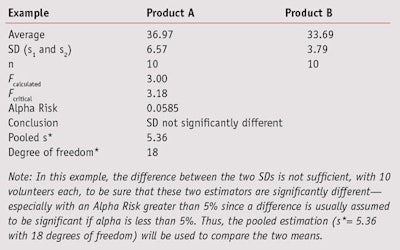
or the Alpha Risk level can be calculated using the Fisher Microsoft Excel Function. In this equation, n1 and n2 are the two sample sizes and F0.95 is the critical value for 95% confidence.6 In the case of pooled estimations (s*), the SD will be calculated as shown in Equation 3 to compare the means.

If Fcalculated is less than Fcritical, the two SDs are assumed to not be significantly different. However, if Fcalculated is greater than Fcritical, the two standard deviations are assumed to be significantly different and will be taken into account separately for the means comparison (see Table 6). In this example, the difference between the two SDs is not sufficient to be sure that these two estimators are significantly different. Thus, the pooled estimation (s*= 5.36 with 18 degrees of freedom) will be used to compare the two means.
Considering these two possible conclusions, i.e. that the SDs either can be pooled or they are significantly different, the mean comparison will be investigated according two different approaches: one where two data sets have comparable SDs, and another where two data sets present significantly different SDs.
Comparable SDs: To compare two data sets having comparable SDs, the standard Student’s t-test can be performed using Equation 4,
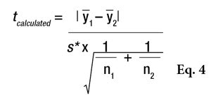
where Ῡ1 and Ῡ2 are the two sample averages. This t-statistic must also be compared to a critical value, via Equation 5

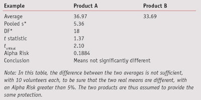
or the Alpha Risk level can be calculated using the Student Microsoft Excel Function. If the tcalculated is greater than tcritical, the two means are assumed to be significantly different (see Table 7). In this table, the difference between the two averages is not sufficient to be sure that the two real means are different. The two products are thus assumed to provide the same protection.
Significantly different SDs: In the case of two data sets presenting significantly different standard deviations, a Welch’s W-test should be used, which is the most rigorous test; however, it is poorly known and less often used because the statistical tables required to interpret the results are difficult to find. Therefore, it is usually replaced by a modified Student’s t-test according to Equation 6.
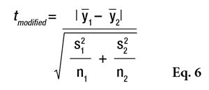
If tmodified is greater than tcritical, the two means are assumed to be significantly different. This t-statistic also must be compared with a critical value (see Eq. 5) or the Alpha Risk can be calculated using the Student Microsoft Excel Function. Readers should note that if normality is not assumed, the two data sets could be compared using the Wilcoxon’s nonparametric Rank-sum test.7 As a cautionary note, when the t-test concludes that two products are significantly different, the exact level of risk is known but if the sample size increases or a new test is conducted, the conclusion has a low level of probability of being different, i.e., less than the calculated risk. On the other hand, if the tests cannot conclude that the two products are different, another kind of risk is present: the conclusion that the two products are similar is wrong. In this case, it may be possible to estimate the greatest difference between the two products according the accuracy of the measurements. In the case of a comparison based on 10 volunteers, the gap between the two products cannot be greater than 3*σ/√5, otherwise there would be a greater than 90% chance of it being detected.8 In the example given in Table 7, it could not be proven that there was an effect related to the formula change (lag = 3.3 and alpha = 0.1884) but if there was, it would certainly be less than 7.2 (3*5.36/√5), otherwise it would have been detected. Put another way, the modified formula would result in a maximum variation of 7.2 SPF points.
When comparing the estimated SPF with a claimed SPF, the approach is different. The product developer is confronted with the comparison of an estimated value over a specified value and is not comparing two estimated averages; in this case, the gap is only 3*σ/√10. For example, with product B, with a standard deviation of 5.36 based on 10 volunteers, it would have required the actual gap in the claim to be at least 5 in order to be detected, meaning a real SPF of 35. With the SPF of product B measured at 33.69, the risk of claiming the product to have an SPF of 30 is too high. This was also demonstrated by the confidence interval.
Test Subjects
The methods for determining the SPF in vivo are clear; a minimum of 10 valid results is only sufficient if the 95% CI of the mean SPF is within +17% of the mean SPF. Otherwise, the number of subjects is increased stepwise from 10, and up to a maximum of 20 valid results from a maximum of 25 subjects until the statistical criteria are met. If the statistical criteria have not been met after 20 valid results from the maximum 25 subjects, the test should be rejected.4
It is obvious that this method is time-consuming and impractical but as mentioned, throughout the development of a sunscreen, it is necessary to verify the SPF value of the product so that it is in line with the claimed SPF. While using an in vitro method is recommended,9-11 it also is possible to use the in vivo method with a reduced number of volunteers. However, when reducing the panel from 10 volunteers to just 5, it is important to consider the impact in terms of statistical uncertainty. This reduction allows for a slightly faster result and reduces the costs of developing the formula. The results should then be confirmed by more advanced tests using at least 10 volunteers.
Once again, statistics can serve as a helpful tool to facilitate decision-making regarding the product’s development. The 95% CI semi-range for a result on 10 volunteers (under the normality hypothesis) is expressed by Equation 7.

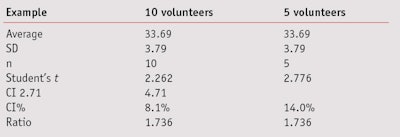
Considering that with five volunteers the standard deviation will not change, one could estimate what this HR could be for an average of five volunteers (see Figure 1 and Table 8). According to the normal law, the average should not be impacted by the change from 10 to 5 volunteers; however, the main effect observed will be in the confidence interval, where the uncertainty will increase by 73.6% and the SPF range in this example will change from 33.69 + 2.7 to 33.69 + 4.7 (see Table 8).
In contrast, it is also interesting to estimate the CI of 10 volunteers based on the values obtained from 5 volunteers. This allows product developers to simulate the values obtained with a minimum of 10 volunteers for the validation of sun products. This calculation is achieved by Equation 8.

Meeting the Claimed SPF Goal
Thanks to this approach, an abacus has been established that can answer the following question: When developing a formula, which average and SD pair could the product developer consider as having a high enough probability to reach the claimed SPF goal? To determine this level of confidence and thus avoid further statistical calculations, a graphical representation is proposed based on the difference (Δ) in the pair’s estimated and claimed SPF and SEM, which allows for the estimation of in which area the confidence is located to be superior to the claim. To determine the probability of the real SPF being higher than target, a) the difference between the observed SPF mean and targeted SPF mean is calculated, then b) the SEM (SEM = SD/√(number of volunteers)) is calculated. At the location of this pair of values—i.e., the a value on the x-axis and the b value on the y axis, the confidence in the difference is given according to a one-sided Student’s t-test.
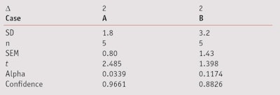
Consider an example report given by an institute, which gave the following results. Product B has a mean SPF = 17, an SD = 3.2, and n = 5. According to the mean SPF, the target should be 15. So, what is the confidence associated with this potential claim? The difference (Δ), in this case 17 – 15 = 2; and since SEM = SD/√n, in this case 3.2/√5 = 1.43. Figure 2 shows that the confidence for this claim is between 85–90% (88.26%, according to student table and Table 9), therefore the claim cannot be made without too high a level of risk, since a minimum 95% confidence is necessary to be sure the product SPF is in fact greater than the claimed SPF.
If the SD had been lower, such as with product A having an SD = 1.8 and the same Δ = 2, the confidence should have been greater than 95% (SEM = 0.8), as shown in Table 9, and thus the product developer could be confident in concluding the claimed SPF has been reached. Given that these assessments for products A and B were made with 5 volunteers, it is interesting to predict the confidence level for 10 volunteers using the same mean and SD. Applying the same principle of calculation as before,8 one can derive the chart shown in Figure 3.
This figure estimates the confidence levels in SPF claims calculated for 10 volunteers based on the results observed for 5 volunteers. Due to the fact that below an SPF of 30, the claims are classified by steps of 5, the gap between the measured SPF and the claim cannot exceed 4.99. Figure 3 also shows that below an SEM of 4, researchers can be confident with the hypothesis that the SPF should be greater than the revendication. In other words, researchers can launch the official validity test on 10 volunteers with an acceptable level of risk. In all other cases, it should be preferable to improve the formula.
Conclusions
The methods for determining sun protection factors in vivo are based, by definition, on a biological response of the human skin. To overcome the intrinsic variation of these methods, it is essential to use a large number of volunteers and therefore involve statistics but unless these concepts are used every day, they often are poorly understood or worse, misinterpreted. This article discusses how these values should be interpreted and explains what they mean to formulators. For example, it was remarkable to see the effects of reducing the number of volunteers from 10 to 5; according to the normal distribution law, the average does not change significantly but the %CI increases by 73%.
In addition, the authors devised a method to estimate the maximum deviation, which is a value that cannot be detected and thus a point rarely mentioned in cosmetics. This is a second type of risk that allows researchers to draw conclusions in the absence of significant effects.
Further, a method to calculate the test results for 5 volunteers based on SPF and its SD is proposed to determine the risk that can be taken for claiming an SPF that is different from the average SPF. For SPFs of 6 to 30, with 5 volunteers, the maximum difference between the observed and the claimed value cannot exceed 4.99 points and the SEM should therefore not exceed 3.8 to maintain confidence in the hypothesis that the SPF measured on 10 volunteers will be greater than the revendication. Finally, these calculations are depicted graphically as a tool for product developers to judge whether to continue the development of a product based on the results of the screening tests on 5 volunteers, or to adjust the formulation before continuing the project.
References
Send e-mail to [email protected].
1. European commission recommendation on the efficacy of sunscreen products and the claims made relating thereto, available at https://eur-lex.europa.eu/LexUriServ/LexUriServ.do?uri=OJ:L:2006:265:0039:0043:en:PDF (Accessed Jan 19, 2011)
2. Colipa recommendations N21–23, available at: www.colipa.eu/publications-colipa-the-european-cosmetic-cosmetics-association/recommendations.html (Accessed Jan 3, 2011)
3. www.fda.gov/ohrms/dockets/98fr/07-4131.pdf (Accessed Jan 3, 2011)
4. Colipa website, 2006 International Sun Protection Factor (SPF) Test Method, available at www.colipa.eu/publications- colipa-the-european-cosmetic-cosmetics-association/guidelines.html?view=item&id=21%3Ainternational-sun-protection-factor-spf-test-method-2006-cd-rom-included&catid=46%3Aguidelines (Accessed Jan 3, 2011)
5. A Hald, in Statistical Tables and Formulas, John Wiley and Sons, New York (1952)
6. RA Fisher and F Yates, in Statistical Tables for Biological, Agricultural and Medical Research, Oliver and Boyd, London (1963)
7. F Wilcoxon, Individual comparisons by ranking methods, Biometrics 1 80–83 (1945)
8. E Morice, Puissance de quelques tests classiques effectif d’echantillon pour des risques alpha fixés, Revue de Statistique Appliquée 16 1 77–126 (1968) 9. M Pissavini et al, Determination of the in vitro SPF, Cosmet & Toil 118, 63–72 (2003)
10. L Fageon, D Moyal, J Coutet and D Candau, Importance of sunscreen products spreading protocol and substrate roughness for in vitro sun protection factor assessment, Int J Cosmet Sci 31 6 405–418 (2009)
11. PJ Matts et al, The COLIPA in vitro UVA method: A standard and reproducible measure of sunscreen UVA protection, Int J of Cosm Sci 32, 35-46 (2010)
Lab Practical: Statistics Translated
- The arithmetic average of SPF values indicates what the real SPF value could be.
- The standard deviation of SPF values gives an indication of a pool of heterogeneity between consumer SPF results and uncertainty on measurements.
- The CI of SPF values gives an indication of the area in which the real SPF is assumed to be.
- During sunscreen product development, the obtained SPF value is compared with the values of previous batches according to the mean SPF value and its standard deviation.



!['[Sunscreen] developers will be able to innovate more efficiently while maintaining high standards of quality and safety for consumers.'](https://img.cosmeticsandtoiletries.com/files/base/allured/all/image/2024/06/woman_outside_using_sunscreen_on_face_ISO_test_standards_AdobeStock_783608310.66678a92029d9.png?auto=format%2Ccompress&fit=crop&h=191&q=70&rect=62%2C0%2C2135%2C1200&w=340)
